단단한 강화학습 코드 정리, chap10
단단한 강화학습 책의 코드를 공부하기 위해 쓰여진 글이다.
Tile Coding
1
2
3
4
# Following are some utilities for tile coding from Rich.
# To make each file self-contained, I copied them from
# http://incompleteideas.net/tiles/tiles3.py-remove
# with some naming convention changes
IHT
1
2
3
4
5
6
7
8
9
10
11
12
13
14
15
16
17
18
19
20
21
22
23
24
25
26
27
28
class IHT:
    "Structure to handle collisions"
    def __init__(self, size_val):
        self.size = size_val
        self.overfull_count = 0
        self.dictionary = {}

    def count(self):
        return len(self.dictionary)

    def full(self):
        return len(self.dictionary) >= self.size

    def get_index(self, obj, read_only=False):
        d = self.dictionary
        if obj in d:
            return d[obj]
        elif read_only:
            return None
        size = self.size
        count = self.count()
        if count >= size:
            if self.overfull_count == 0: print('IHT full, starting to allow collisions')
            self.overfull_count += 1
            return hash(obj) % self.size
        else:
            d[obj] = count
            return count
- (1) : 타일 코딩을 위한 해시값을 구하는 함수
- (3~6) : 클래스의 생성자
self.size = size_val: 인덱스의 최댓값(=인덱스의 개수)self.overfull_count: key 값이 꽉찼는데 hash 함수를 호출한 횟수self.dictionary: 해시의 key, value를 저장하는 해시테이블
- (8~9) : 해시테이블의 key 의 개수를 반환하는 메소드
- (11~12) : 해시테이블의 key 개수가 지정된 size 이상인지를 확인하는 함수
- (14) : 해시값을 반환하는 메소드
obj: 해시값을 구하게 될 대상 객체read_only: True일 경우 읽기만 하며 해시테이블에 key 값이 없으면 None을 반환한다. False일 경우 key 값에 해당하는 Value 값을 만들고 해당 값을 해시테이블에 저장하고 해당 값을 반환한다..
- (15) : 클래스 변수
self.dictionary를d에 저장한다. - (16~17) : 해시테이블에 key가 존재할경우 해당 key의 value를 반환한다.
- (18~19) :
read_only가True일 경우 읽기만 하므로 바로None을 반환한다. - (20~21) : 해시테이블의 사이즈와 해시테이블에 저장된 key의 개수를 각각
size,count에 저장한다. - (22~25) : 해시테이블의 key의 개수가 size 이상일 경우
self.overfull_count를 1 증가시키고obj의 파이썬 내부 해시값의size의 나머지를 반환한다. - (26~28) : 해시테이블이 꽉 차있지 않으면 현재 key의 개수를 value로 하여 값을 반환한다.
- 요약 : 먼저 온 것부터 1, 2, 3 채우다가 다 차면
hash(obj) % size를 반환한다.
hash_coords
1
2
3
4
def hash_coords(coordinates, m, read_only=False):
    if isinstance(m, IHT): return m.get_index(tuple(coordinates), read_only)
    if isinstance(m, int): return hash(tuple(coordinates)) % m
    if m is None: return coordinates
- (1) : 해시값을 반환하는 함수이다
coordinates: 해시값을 산출하기 위한 정수 리스트m: 해시의 종류,IHT클래스의 인스턴스 혹은 정수값이다.read_only: True일 경우 읽기만 하며 해시테이블에 key 값이 없으면 None을 반환한다. False일 경우 key 값에 해당하는 Value 값을 만들고 해당 값을 해시테이블에 저장하고 해당 값을 반환한다..
- (2) :
m이IHT클래스의 인스턴스일 경우get_index메소드를 이용하여 해시값을 반환한다. - (3) :
m이 정수일 경우coordinates의 튜플값의 해시값(파이썬 해시함수 사용)의 나머지를 반환한다. - (4) :
m이None일 경우coordinates를 그대로 반환한다.
tiles
1
2
3
4
5
6
7
8
9
10
11
12
13
14
15
16
def tiles(iht_or_size, num_tilings, floats, ints=None, read_only=False):
    """returns num-tilings tile indices corresponding to the floats and ints"""
    if ints is None:
        ints = []
    qfloats = [floor(f * num_tilings) for f in floats]
    tiles = []
    for tiling in range(num_tilings):
        tilingX2 = tiling * 2
        coords = [tiling]
        b = tiling
        for q in qfloats:
            coords.append((q + b) // num_tilings)
            b += tilingX2
        coords.extend(ints)
        tiles.append(hash_coords(coords, iht_or_size, read_only))
    return tiles
- (1~2) : 수들을 받고 그에 해당하는 tile 인덱스들을 반환하는 함수
iht_or_size:IHT클래스 또는 정수값을 인수로 받아hash_coords에서 해당 인스턴스에 해당하는 해시값을 구한다.num_tilings: 반환하는 타일 인덱스의 개수floats: 상태를 표현하는 정규화된 실수, 여기서는 (위치, 속도)로 표현된다.ints: 행동을 표현하는 정수, 여기서는 -1, 0, 1 중 하나가 된다.read_only: True일 경우 읽기만 하며 해시테이블에 key 값이 없으면 None을 반환한다. False일 경우 key 값에 해당하는 Value 값을 만들고 해당 값을 해시테이블에 저장하고 해당 값을 반환한다..
- (3~4) :
ints가None일 경우ints를 빈 리스트로 초기화한다. 상태 가치만 얻고 싶다면ints를None으로 하여 근사할 수 있다. 예시에서는 행동도 같이 제공하므로 해당하지 않는다. - (5) : 상태를 나타내는
floats의 실수값들에num_tilings를 곱한 후 내림하여 정수로 만든다. quantize의 q가 아닐까 싶다. - (6) : 반환할 tile의 인덱스를 저장하는 빈 리스트를 생성한다.
- (7) :
num_tilings횟수만큼 반복하며 반복마다 한 해시값을tiles에 추가한다.tiling은 반복 변수이다. - (8) : 0부터 시작하는 반복변수
tiling에서 2를 곱한 값을 저장한다. - (9) :
coords리스트에 반복변수tiling을 넣고 초기화한다. - (10) :
b에 반복변수tiling을 저장한다. - (11~13) : 각
qfloats의 값(상태에 타일의 개수를 곱한 후 내림한 값)에 b를 더하고 타일의 개수로 나눈후 내림한 값을coords리스트에 추가한다. b에tilingX2(tiling반복변수에 2를 곱한 값)를 더한다. -
\[K_j =\lfloor \frac{Q_j + (i + 2 \times (j-1))}{\vert T \vert} \rfloor\]
- $K$ : coords에 추가되는 숫자들
- $\vert T \vert$ : number of tiles
- $Q_j$ : $\lfloor S_j \times \vert T \vert \rfloor$
- $i$ : index of tile
- $j$ : index of state
- (14) :
coords에ints를 추가한다. 이러면coords는 [index of tile] + $K$ + [ints] 가 된다. - (15) :
coords,iht_or_size,read_only값을 기반으로 얻은 해시값을tiles리스트에 추가한다. - (16) :
num_tilings개수 만큼 타일 인덱스를 가진tiles를 반환한다.
mountain_car
1
2
3
4
5
6
7
8
9
10
11
12
13
14
15
16
17
18
19
20
21
22
23
24
25
26
27
# all possible actions
ACTION_REVERSE = -1
ACTION_ZERO = 0
ACTION_FORWARD = 1
# order is important
ACTIONS = [ACTION_REVERSE, ACTION_ZERO, ACTION_FORWARD]

# bound for position and velocity
POSITION_MIN = -1.2
POSITION_MAX = 0.5
VELOCITY_MIN = -0.07
VELOCITY_MAX = 0.07

# use optimistic initial value, so it's ok to set epsilon to 0
EPSILON = 0

# take an @action at @position and @velocity
# @return: new position, new velocity, reward (always -1)
def step(position, velocity, action):
    new_velocity = velocity + 0.001 * action - 0.0025 * np.cos(3 * position)
    new_velocity = min(max(VELOCITY_MIN, new_velocity), VELOCITY_MAX)
    new_position = position + new_velocity
    new_position = min(max(POSITION_MIN, new_position), POSITION_MAX)
    reward = -1.0
    if new_position == POSITION_MIN:
        new_velocity = 0.0
    return new_position, new_velocity, reward
- (1~4) : 가속 방향을 나타내는 변수
ACTION_REVERSE: 뒷방향(왼쪽)ACTION_ZERO: 아무 행동도 하지 않음ACTION_FORWARD: 정면(오른쪽)
- (5~6) : 행동들을 저장하는 리스트, (←, ·, →) 순서로 저장된다
- (8~12) : 위치와 속도의 경계값
- 위치 : $[-1.2, 0.5]$
- 속도 : $[-0.7, 0.7]$
- (14~15) : ε-greedy 정책을 위한 ε의 값을 결정한다. 최적의 초기값을 설정하므로 ε을 0으로 설정한다, (보상이 무조건 -1이므로 상태 또는 상태-액션 가치가 0을 넘을 수 없다, 이 경우 모든 action에 대해 충분한 탐색을 할 수 있다.) ε이 0일 경우 이는 greedy-policy와 같다.
- (17~19) : (위치, 속도, 행동)을 받아 (다음 위치, 다음 속도, 보상)을 반환한다.
- $v$ : 속도, $a$ : 행동(-1, 0, 1), $p$ : 위치
- (20) : $v_{t+1} \leftarrow v_t + 0.001a_t - 0.0025\cos(3p_t)$
- (21) : $v_{t+1} \leftarrow \text{clip}(v_{t+1}, -0.07, 0.07)$
- (22) : $p_{t+1} \leftarrow p_t + v_{t+1}$
- (23) : $p_{t+1} \leftarrow \text{clip}(p_{t+1}, -1.2, 0.5)$
- (24) : 보상은 언제나 -1이다.
- (25) : 맨 왼쪽에 도달할 경우 속도를 0으로 만든다.
- (27) : 새로운 위치, 새로운 속도, 보상을 반환한다.
ValueFunction
1
2
3
4
5
6
7
8
9
10
11
12
13
14
15
16
17
18
19
20
21
22
23
24
25
26
27
28
29
30
31
32
33
34
35
36
37
38
39
40
41
42
43
44
45
46
47
48
49
50
51
52
53
54
# wrapper class for state action value function
class ValueFunction:
    # In this example I use the tiling software instead of implementing standard tiling by myself
    # One important thing is that tiling is only a map from (state, action) to a series of indices
    # It doesn't matter whether the indices have meaning, only if this map satisfy some property
    # View the following webpage for more information
    # http://incompleteideas.net/sutton/tiles/tiles3.html
    # @max_size: the maximum # of indices
    def __init__(self, step_size, num_of_tilings=8, max_size=2048):
        self.max_size = max_size
        self.num_of_tilings = num_of_tilings

        # divide step size equally to each tiling
        self.step_size = step_size / num_of_tilings

        self.hash_table = IHT(max_size)

        # weight for each tile
        self.weights = np.zeros(max_size)

        # position and velocity needs scaling to satisfy the tile software
        self.position_scale = self.num_of_tilings / (POSITION_MAX - POSITION_MIN)
        self.velocity_scale = self.num_of_tilings / (VELOCITY_MAX - VELOCITY_MIN)

    # get indices of active tiles for given state and action
    def get_active_tiles(self, position, velocity, action):
        # I think positionScale * (position - position_min) would be a good normalization.
        # However positionScale * position_min is a constant, so it's ok to ignore it.
        active_tiles = tiles(self.hash_table, self.num_of_tilings,
                            [self.position_scale * position, self.velocity_scale * velocity],
                            [action])
        return active_tiles

    # estimate the value of given state and action
    def value(self, position, velocity, action):
        if position == POSITION_MAX:
            return 0.0
        active_tiles = self.get_active_tiles(position, velocity, action)
        return np.sum(self.weights[active_tiles])

    # learn with given state, action and target
    def learn(self, position, velocity, action, target):
        active_tiles = self.get_active_tiles(position, velocity, action)
        estimation = np.sum(self.weights[active_tiles])
        delta = self.step_size * (target - estimation)
        for active_tile in active_tiles:
            self.weights[active_tile] += delta

    # get # of steps to reach the goal under current state value function
    def cost_to_go(self, position, velocity):
        costs = []
        for action in ACTIONS:
            costs.append(self.value(position, velocity, action))
        return -np.max(costs)
- (1~7) : 상태 행동 가치 함수를 표현하기 위한 클래스이다. 타일링은 (state, action)를 인덱스 시리즈에 대응시킨다. 대응이 몇개의 속성을 만족한다면 인덱스가 의미를 가지는지는 중요하지 않다.
- (8~9) : 클래스의 생성자이다.
step_size: 시간 간격을 의미하며 $\alpha$로 표기된다.num_of_tilings: (state, action)마다 대응되는 인덱스의 개수max_size: 인덱스의 최댓값(=개수)
- (10~11) : 인수로 들어온
num_of_tilings,max_size를 클래스 변수에 저장한다. - (13~14) : 인수로 들어온
step_size를 타일의 개수로 나누어 클래스 변수에 저장한다. - (16) : 타일링을 위한 해시 값을 구하기 위한 IHT(Index Hash Table) 클래스를 선언하고 클래스변수에 저장한다.
- (18~19) : 가치함수를 근사하기 위한 함수 가중치를 0으로 초기화한다. (각 타일의 가중치)
- (21~23) : tile coding을 위해 스케일링 값을 저장한다.
position_scale: $\vert T \vert / (p_{\max} - p_{\min})$velocity_scale: $\vert T \vert / (v_{\max} - v_{\min})$
- (25~26) : (위치, 속도, 행동)을 받아 그에 해당하는 활성화 타일들(8개) 반환하는 함수이다.
- (27~28) :
positionScale * (position - position_min)으로 하면 범위가 $[0, 8]$로 된다. 근데positionScale * position_min은 상수이므로 이를 제외해도 된다는 것이다. 제외할 경우 범위는 약 $[-5.65, 2.35]$가 된다. - (29~31) :
tiles에 해시테이블, 타일의 개수, 정규화된 위치와 속도, 행동을 넣고 활성화된 타일들을 얻는다. (num_of_tiling만큼) - (32) : 활성화된 타일들을 반환한다.
- (34~35) : (위치, 속도, 행동) 쌍에 해당하는 추정가치를 반환하는 함수이다, 수식으로 나타내면 $\hat{q}(S, A, \textbf{w})$로 나타낼 수 있다.
- (36~37) : 목표 위치(
POSITION_MAX)에 도달한 상태이면 0을 반환한다. - (38) :
get_active_tiles메소드를 통해 활성화된 타일들을 얻는다. - (39) : 활성화된 타일들의 가중치를 모두 더한 값을 반환한다.
- (41~42) : $S, A, G$(상태, 행동, 목표)로 가치함수($\textbf{w}$)를 학습한다.
- (43~44) :
self.get_active_tiles를 통해 활성화된 타일들을 얻고 이를 토대로 추정치($\hat{q}(S, A, \textbf{w})$)를 얻는다. - (45) : $\textbf{w}$를 갱신하기 위한 업데이트 양인 delta 값을 얻는다.
- $\text{delta} = \alpha \left [ G - \hat{q}(S_{\tau}, A_{\tau}, \textbf{w})\right ]\nabla\hat{q}(S_{\tau}, A_{\tau}, \textbf{w})$
- 활성화된 타일들의 가중치가 1이기 때문에 $\nabla \hat{q}$는 생략된다.
- (46~47) : 활성화된 타일들만 delta 값을 더해서 갱신한다. 활성화되지 않은 타일들은 가중치가 0이므로 활성화된 타일들만 더해서 갱신한다.
- $\textbf{w} \leftarrow \textbf{w} + \alpha \left [ G - \hat{q}(S_{\tau}, A_{\tau}, \textbf{w})\right ]\nabla\hat{q}(S_{\tau}, A_{\tau}, \textbf{w})$
- (49~50) : 현재 상태 가치함수를 기반으로 현재 상태에서 목표 도달까지 몇 스텝이 필요한지 계산하는 메소드, 보상이 무조건 -1이고 $\gamma=1$이므로 가치값이 곧 스텝의 값이다.
- (51) : 각 행동별 스텝의 개수를 저장하는 리스트
- (52~53) : 각 행동별로 가치를 구해서
costs리스트에 추가한다. - (54) : 가치값은 모두 음수이므로 그중에 가장 큰 값(스텝이 가장 적은 값)을 -1을 곱해 양수로 바꾼 후 반환한다.
get_action
1
2
3
4
5
6
7
8
# get action at @position and @velocity based on epsilon greedy policy and @valueFunction
def get_action(position, velocity, value_function):
    if np.random.binomial(1, EPSILON) == 1:
        return np.random.choice(ACTIONS)
    values = []
    for action in ACTIONS:
        values.append(value_function.value(position, velocity, action))
    return np.random.choice([action_ for action_, value_ in enumerate(values) if value_ == np.max(values)]) - 1
- (1~2) :
position,velocity에서 ε-greedy 정책과value_function에 기반하여 행동을 결정하는 함수 - (3~4) : ε의 확률로 무작위로 행동을 선택한다.
- (5~7) : 가능한 모든 행동들의 가치를 산출하여
values리스트에 저장한다. - (8) : 최댓값을 가진 행동들 중 임의로 하나를 반환한다.
np.argmax를 사용하면 최댓값이 여러 개 있을 때 첫 번째 인덱스를 반환하므로, 가치가 최대인 행동들 중 하나를 임의로 선택하는 코드를 사용한다.if value_ == np.max(values):values의 요소값인value_가values_의 최댓값과 같다면action_ for action_, value_ in enumerate(values): 행동의 인덱스를 배열에 추가한다.np.random.choice(...): 배열에 들어간 행동중에 하나를 무작위로 선택한다.np.random.choice(...) - 1:action_은 [0, 1, 2]이고 실제 행동은 [-1, 0, 1] 이므로 선택된 행동에서 1을 빼준다.
semi_gradient_n_step_sarsa
1
2
3
4
5
6
7
8
9
10
11
12
13
14
15
16
17
18
19
20
21
22
23
24
25
26
27
28
29
30
31
32
33
34
35
36
37
38
39
40
41
42
43
44
45
46
47
48
49
50
51
52
53
54
55
56
57
58
59
60
61
62
63
# semi-gradient n-step Sarsa
# @valueFunction: state value function to learn
# @n: # of steps
def semi_gradient_n_step_sarsa(value_function, n=1):
    # start at a random position around the bottom of the valley
    current_position = np.random.uniform(-0.6, -0.4)
    # initial velocity is 0
    current_velocity = 0.0
    # get initial action
    current_action = get_action(current_position, current_velocity, value_function)

    # track previous position, velocity, action and reward
    positions = [current_position]
    velocities = [current_velocity]
    actions = [current_action]
    rewards = [0.0]

    # track the time
    time = 0

    # the length of this episode
    T = float('inf')
    while True:
        # go to next time step
        time += 1

        if time < T:
            # take current action and go to the new state
            new_position, new_velocity, reward = step(current_position, current_velocity, current_action)
            # choose new action
            new_action = get_action(new_position, new_velocity, value_function)

            # track new state and action
            positions.append(new_position)
            velocities.append(new_velocity)
            actions.append(new_action)
            rewards.append(reward)

            if new_position == POSITION_MAX:
                T = time

        # get the time of the state to update
        update_time = time - n
        if update_time >= 0:
            returns = 0.0
            # calculate corresponding rewards
            for t in range(update_time + 1, min(T, update_time + n) + 1):
                returns += rewards[t]
            # add estimated state action value to the return
            if update_time + n <= T:
                returns += value_function.value(positions[update_time + n],
                                                velocities[update_time + n],
                                                actions[update_time + n])
            # update the state value function
            if positions[update_time] != POSITION_MAX:
                value_function.learn(positions[update_time], velocities[update_time], actions[update_time], returns)
        if update_time == T - 1:
            break
        current_position = new_position
        current_velocity = new_velocity
        current_action = new_action

    return time
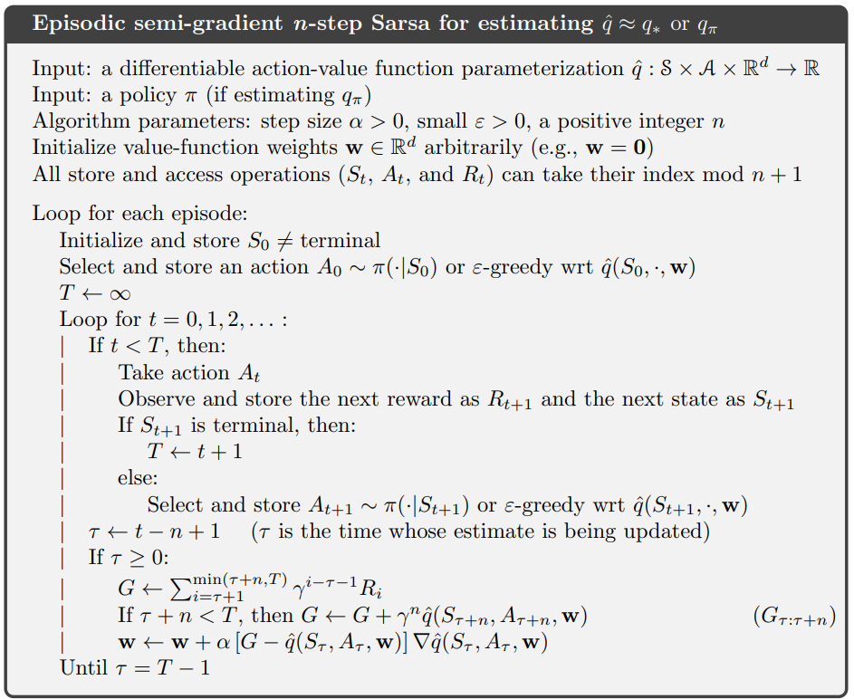
- (1~4) : 준경사도 n-step 살사 알고리즘
value_function: 학습할 상태 가치 함수n: 스텝의 개수
- (5~8) :
current_position에 $[-0.6, -0.4]$ 범위의 균등분포에서 추출한 초기 위치를 대입하고current_velocity에 초기 속도 0을 대입한다.- $\text{Initialize and store }S_0 \neq \text{ terminal}$
- (9~10) :
current_action에 초기 상태를 바탕으로get_action함수를 통해 행동을 얻는다.- $\text{Select and store an action }A_0 \sim \pi(\cdot \vert S_0)\text{ or }\varepsilon\text{-greedy wrt }\hat{q}(S_0, \cdot, \textbf{w})$
- (12~16) : 상태(위치, 속도), 행동, 보상의 trajectory를 저장하는 리스트를 각각 만든다. mod를 이용해 메모리를 절약할 수 있지만 구현의 편의성을 위해 모두 저장한다.
- $\text{All store and access operations }(S_t, A_t,R_t)\text{ can take their index mod }n + 1$
- (18~19) : 현재 시간을 나타내는 변수, $t$
- (21~22) : 에피소드의 길이 $T$를 $\infty$로 초기화한다. 나중에 terminal state에 도달하면 $T$에 $t+1$을 대입한다.
- $T \leftarrow \infty$
- (23~25) :
time변수를 하나씩 증가시키면서 반복한다. 무한반복인 것 같지만 (39~40) 과 (57~58) 의 종료조건에 의해 종료된다.- $\text{Loop for }t = 0, 1, 2,… :$
- 의사코드에서는 $t=0$ 부터 시작하지만 코드에서는 반복 시작시에
time += 1연산을 하므로 1부터 시작하고 반복문 내부에서time이 알고리즘의 $t$보다 1이 크다는 차이가 있다.
- (27) : 종료시점 전까지 행동을 수행한다.
- $\text{If } t < T,\text{ then:}$
- (28~40) : 현재 (상태, 행동)에 대해 새로운 (상태, 행동, 보상)을 받는다. 정책에 따라 새로운 상태에 대해
get_action으로 다음 행동을 얻고 새로운 (상태, 행동, 보상)을 각각 리스트에 저장한다. 새로운 상태가 terminal state라면T에time을 대입한다. (23~25) 에서 말한 것과 같이 현 상태에서time은 $t+1$이므로time을 그대로 대입한다.
- (42~43) : 업데이트(학습)될 시간을 구한다
- $\tau \leftarrow t-n+1$
- $(\tau\text{ is the time whose estimate is being updated})$
- (44) : 업데이트될 시간이 0보다 크면 학습을 시작한다.
- $\text{If }\tau \geq 0$
- (45) : 코드 구현적으로 이득을 추정할 변수를 0으로 초기화한다.
- (46~48) : n-step만큼의 보상을 누적한다. 여기서 $\gamma=1$이다
update_time+1(reward[0]은 0으로 초기화됬기 때문) 부터T또는update_time+n까지returns에 더한다.update_time+n까지 더할 경우n개를 더하게 된다.- $G \leftarrow \sum_{i=\tau+1}^{\min(\tau+n, T)}\gamma^{i-\tau-1}R_i$
- (49~53) :
update_time의 n-스텝 이후가 terminal state가 아닐 경우 n-스텝 이후의 가치를 더한다.- $\text{If }\tau+n<T\text{, then }G \leftarrow G + \gamma^{n}\hat{q}(S_{\tau+n}, A_{\tau+n}, \textbf{w})$
- (54~56) :
returns과 현재 상태, 행동을 이용하여 가치함수의 가중치를 갱신한다.- $\textbf{w} \leftarrow \textbf{w} + \alpha \left [ G - \hat{q}(S_{\tau}, A_{\tau}, \textbf{w})\right ]\nabla\hat{q}(S_{\tau}, A_{\tau}, \textbf{w})$
- (57~58) : 업데이트될 시간이 종료시점 바로 전이면 반복을 종료한다.
- $\text{Until } \tau=T-1$
- (59~61) : 새로운 상태와 행동을 갱신한다.
- (63) : 에피소드 종료까지 소요된 시간을 반환한다.
figure_10_2
1
2
3
4
5
6
7
8
9
10
11
12
13
14
15
16
# Figure 10.2, semi-gradient Sarsa with different alphas
def figure_10_2():
    runs = 10
    episodes = 500
    num_of_tilings = 8
    alphas = [0.1, 0.2, 0.5]

    steps = np.zeros((len(alphas), episodes))
    for run in range(runs):
        value_functions = [ValueFunction(alpha, num_of_tilings) for alpha in alphas]
        for index in range(len(value_functions)):
            for episode in tqdm(range(episodes)):
                step = semi_gradient_n_step_sarsa(value_functions[index])
                steps[index, episode] += step

    steps /= runs
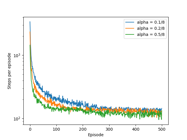
- (1~2) : step size($\alpha$) 별로 Mountain Car 환경에서 에피소드가 진행될 수록 Goal 도달까지 step의 개수의 변화를 그린다.
- (3~4) : 독립적인 10번 실행하고 한번의 실행당 500번의 에피소드를 진행한다. 각 에피소드별로 10번의 실행이있을텐데 그것을 평균해서 플로팅한다.
- (5) : 타일의 개수를 8개로 한다.
- (6) : 각각 다르게 할 step size, 0.1, 0.2, 0.5로 설정한다.
- (8) : 각 $\alpha$값을 행으로 하고 각 에피소드의 시점을 열로 하는 행렬을 만든다.
value[a][b]는a번째 인덱스의 step size로 학습시b번째 에피소드에서는 목표 도달까지value[a][b]번의 스텝이 소요된다는 뜻이다. - (9) : 독립적인 10번의 실행을 한다.
- (10) : step size($\alpha$)별로 가치함수를 초기화한다.
- (11) : 각 step size 별로 학습을 시작한다.
- (12) :
episodes번의 에피소드를 실행한다. - (13) : 해당 step size로 진행한 학습의
episode번째 실행에서의 목표까지 도달하는 데 필요한step의 횟수를 저장한다. - (14) :
steps행렬에 누적한다 - (16) :
steps은runs개수만큼step이 누적되어 있으므로 이를 평균하기 위해runs로 나누어준다.