JAX 시행착오/패턴
1.
jnp.inner과 vmap이 같이 활용되다보니 헷갈린 예시 (아래 예시는 최대한 간단히 재구성함)
ndim이 2인 두 행렬을 계산한다고 가정하자 예를 들어 아래와 같다.
1
2
test1 = jnp.arange(0, 6).reshape(3, 2)  # (3, 2)
test2 = jnp.arange(1, 7).reshape(3, 2)  # (3, 2)
여기서 아래 두 연산은 test1, test2에 대해 동작한다.
jnp.innerjax.vmap(jnp.inner)
하지만 결과는 각각 다르다.
1
2
print(jnp.inner(test1, test2).shape)  # (3, 3)
print(jax.vmap(jnp.inner)(test1, test2).shape)  # (3,)
두번째 jax.vmap(jnp.inner)은 axis를 따로 설정하지 않을 경우 axis=0을 배치라고 생각하고 연산하기 때문에 test1, test2는 axis=0 축의 같은 인덱스에 있는 벡터끼리 jnp.inner 연산을 하는 것과 같다.
때문에 2번째 연산의 경우 [ 2, 18, 50] 의 결과가 나오는데 이것은
1
2
3
4
 test1   test2
[[0 1]  [[1 2]
 [2 3]   [3 4]
 [4 5]]  [5 6]]
위와 같은 연산에서
[0*1 + 1*2, 2*3 + 3*4, 4*5 + 5 * 6] 과 같다.
Einstein Summation Convention 으로 표현하면 각 연산은 다음과 같다.
아래 연산은 a.shape == b.shape == (3, 2) 를 기준으로 한다.
jnp.inner:'ij,kj->ik'jax.vmap(jnp.inner):'ij,ij->i'
2. vmap의 2차원 활용
어떤 2차원 배열이 있을 때 axis=0(행) 과 axis=1(열) 의 각 axis의 index에 의존한 연산을 하고싶을 때는 어떻게 해야 할까
먼저 인덱스부터 얻어보자 5 x 4 배열의 모든 요소의 인덱스를 얻고 싶다면
(0, 0), (0, 1), …, (4, 3) 까지 모두 25개로 일반화하면 행의 개수와 열의 개수를 곱한 개수만큼의 인덱스가 필요할 것이다.
그렇다면 다음과 같이 인덱스를 얻을 수도 있다.
1
2
3
4
5
6
7
8
9
10
11
ROW = 5
COL = 4

indices = jnp.arange(ROW * COL)

row_indices, col_indices = jnp.divmod(indices, COL)

print(row_indices)
print(col_indices)
# [0 0 0 0 1 1 1 1 2 2 2 2 3 3 3 3 4 4 4 4]
# [0 1 2 3 0 1 2 3 0 1 2 3 0 1 2 3 0 1 2 3]
그럼 아래와 같이 활용할 수 있다.
1
2
3
4
5
6
7
8
9
10
11
12
13
14
15
16
data = jnp.arange(ROW * COL).reshape(ROW, COL)
print(data)
# [[ 0  1  2  3]
#  [ 4  5  6  7]
#  [ 8  9 10 11]
#  [12 13 14 15]
#  [16 17 18 19]]

result = jax.vmap(lambda x, y: data[x, y])(row_indices, col_indices)
result = result.reshape(ROW, COL)
print(result)
# [[ 0  1  2  3]
#  [ 4  5  6  7]
#  [ 8  9 10 11]
#  [12 13 14 15]
#  [16 17 18 19]]
하지만 위의 경우 두 가지 단점이 있다.
reshape과정이 동반되는 것- 각 축의 요소를 곱한 만큼의 인덱스가 필요하다, 예를 들어 ROW=$r$, COL=$c$ 일 경우 $2 \times r \times c$ 의 인덱스가 필요하다.
- $\prod_i^k n(i)$
- $k$ : dimension(
ndim) - $n(i)$ : $i$ 축의 길이(
len)
- $k$ : dimension(
- $\prod_i^k n(i)$
그렇다면 2차원을 2차원답게 활용하려면 어떻게 해야 할까
결론부터 말하면 다음과 같다.
1
2
3
4
5
6
7
8
9
10
11
12
13
ROW = 5
COL = 4

r_indices = jnp.arange(ROW)
c_indices = jnp.arange(COL)

result = jax.vmap(jax.vmap(lambda x, y: data[x,y], in_axes=(None, 0)), in_axes=(0, None))(r_indices, c_indices)
print(result)
# [[ 0  1  2  3]
#  [ 4  5  6  7]
#  [ 8  9 10 11]
#  [12 13 14 15]
#  [16 17 18 19]]
다르게 활용하고 싶다면 함수를 (r, c, ...)의 파라미터를 받는 다른 함수로 바꾸면 된다.
자세한 동작원리와 주의할 점은 아래에서 서술한다.
2.1. #2의 동작원리와 주의할 점
우리가 주목해야 할 부분은 아래 코드이다. 안부터 자세히 뜯어보자
1
jax.vmap(jax.vmap(lambda x, y: data[x,y], in_axes=(None, 0)), in_axes=(0, None))(r_indices, c_indices)
일단 맨 바깥의 함수는 in_axes=(0, None)이다. 그러면 첫 인자는 axis=0를 탐색하여 축의 각 요소마다 할당된 요소를 사용하겠다는 뜻이다. 두번째 None은 병렬된 축에 걸쳐 모든 요소를 활용하겠다는 뜻이다. 병렬 처리된 개수는 처음 r_indices.shape[0] == 5를 따를 것이다.
따라서 그 안에 있는 in_axes=(None, 0) 으로 정의된 vmap 함수에는 각 인자가 다음과 같이 (vmap 되어) 들어갈 것이다.
1
2
3
4
5
(0, [0, 1, 2, 3])
(1, [0, 1, 2, 3])
(2, [0, 1, 2, 3])
(3, [0, 1, 2, 3])
(4, [0, 1, 2, 3])
이제 감이 올 것이다. 이제 이것은
1
jax.vmap(lambda x, y: data[x,y], in_axes=(None, 0))
이 함수로 들어갈 것인데 0축은 None으로 고정이고 1축은 0을 가지므로 두번째 인자의 0번째 축을 기준으로 vmap이 적용된다.
1
2
3
4
5
(0, [0, 1, 2, 3]) -> (0, 0), (0, 1), (0, 2), (0, 3)
(1, [0, 1, 2, 3]) -> (1, 0), (1, 1), (1, 2), (1, 3)
(2, [0, 1, 2, 3]) -> (2, 0), (2, 1), (2, 2), (2, 3)
(3, [0, 1, 2, 3]) -> (3, 0), (3, 1), (3, 2), (3, 3)
(4, [0, 1, 2, 3]) -> (4, 0), (4, 1), (4, 2), (4, 3)
이러면 이제 각 축의 길이만을 사용하여 모든 요소에 접근하는 방법을 알았다. 처음 접근법과 달리 flatten 이나 reshape 할 필요도 없고 인덱스를 모두 구할 필요도 없다.
주의할 점
in_axes 의 순서에 주의해야 한다. 예를 들어
1
jax.vmap(jax.vmap(lambda x, y: data[x,y], in_axes=(0, None)), in_axes=(None, 0))(r_indices, c_indices)
위와 같이 in_axes의 순서를 바꾸면 인자가 다음과 같이 들어가게 된다.
1
2
3
4
([0, 1, 2, 3, 4], 0) -> (0, 0), (1, 0), (2, 0), (3, 0), (4, 0)
([0, 1, 2, 3, 4], 1) -> (0, 1), (1, 1), (2, 1), (3, 1), (4, 1)
([0, 1, 2, 3, 4], 2) -> (0, 2), (1, 2), (2, 2), (3, 2), (4, 2)
([0, 1, 2, 3, 4], 3) -> (0, 3), (1, 3), (2, 3), (3, 3), (4, 3)
그러면 결과가 다음과 같이 나올 것이다.
1
2
3
4
[[ 0  4  8 12 16]
 [ 1  5  9 13 17]
 [ 2  6 10 14 18]
 [ 3  7 11 15 19]]
즉 transpose된 결과가 나오게 된다. 따라서 vmap을 겹쳐서 사용할 때는 in_axes의 순서에 주의해야 한다.
3. 조건에 따라 fori_loop, while_loop 활용하기
내가 하고싶은 것은 다음과 같았다.
만약 음이 아닌 정수가 주어질 경우 fori_loop을 사용하고 해당 횟수만큼 반복한다. 아니면 None이 주어질 경우 cond_fun이 False가 될 때까지 while_loop을 반복한다.
그런데 내 문제는 다음과 같았다 fori_loop와 while_loop의 문서를 보면
1
2
3
4
5
def fori_loop(lower, upper, body_fun, init_val):
  val = init_val
  for i in range(lower, upper):
    val = body_fun(i, val)
  return val
1
2
3
4
5
def while_loop(cond_fun, body_fun, init_val):
  val = init_val
  while cond_fun(val):
    val = body_fun(val)
  return val
body_fun을 보면 둘의 모양이 다르다.
while_loop:body_fun은val을 받아서val을 반환한다.fori_loop:body_fun은i,val을 받아서val을 반환한다.
이는 같은 body_fun을 두 함수에 사용할 수 없다는 뜻이다. 그렇다고 업데이트 함수를 두 개를 만들 수는 없었다. 나의 경우 반복만 하면 되고 i가 필요하지 않았기 때문에 body_fun(val) 형태만 사용하면 되었다.
이럴 경우에는 body_fun을 wrapping하는 함수를 만들어서 사용하면 된다. 기본 구조는 다음과 같다. 나의 경우는 i를 사용하지 않는 것이 자명했기 때문에 del i 를 했지만 본인이 원하고 싶은 대로 활용해도 된다.
1
2
3
def body_fun_fori(i, values):
    del i
    return body_fun(values)
예시는 다음과 같다.
1
2
3
4
5
6
7
8
def body_fun(x):
    return x + 1

def cond_fun(x):
    return x < 7

def body_fun_fori(i, x):
    return body_fun(x)
1
2
3
4
5
6
def get_result(number):
    if number is None:
        result = jax.lax.while_loop(cond_fun, body_fun, init_val)
    else:
        result = jax.lax.fori_loop(0, number, body_fun_fori, init_val)
    return result
하지만 위 get_result는 jit할 수 없다. jit 하기 위해서는 다음과 같은 방법이 가능할 것이다.
1
2
3
4
5
6
7
8
9
10
@jax.jit
def get_result(number):
    return jax.lax.select(number > 0,
                          jax.lax.fori_loop(0, number, body_fun_fori, init_val),
                          jax.lax.while_loop(cond_fun, body_fun, init_val))

get_result(-1)
# Array(7, dtype=int32, weak_type=True)
get_result(100)
# Array(100, dtype=int32, weak_type=True)
사전에 None을 음수로 바꾸거나 설계자체를 바꿔버릴 수도 있다.
그럼 다음과 같이 None을 조건으로 하면 안될까?
1
2
3
jax.lax.select(number is not None,
                          jax.lax.fori_loop(0, number, body_fun_fori, init_val),
                          jax.lax.while_loop(cond_fun, body_fun, init_val))
이에 대해서는 4.에서 다룬다.
4. jax.lax.select 주의점
다음과 같은 코드가 있다 하자. 이는 3. 조건에 따라… 의 마지막 부분을 설명하기 위해 간소화된 코드이다.
1
2
3
4
5
6
7
8
9
10
11
12
def get3():
    return 3

def hate_none(v):
    if v is None:
        raise ValueError(f"ERROR!: {v}.")
    return v

@jax.jit
def test_none(x):
    result = jax.lax.select(x is None, get3(), hate_none(x))
    return result
hate_none은 None이 들어오면 에러를 발생시키는 함수이다.
test_none 함수를 보면 x가 None이면 get3()을 실행하고 아니면 hate_none(x)를 실행한다.
그럼 우리의 직관상 x가 None일 경우 get3()이 실행되기 때문에 해당 함수는 오류가 일어나지 않을 것 처럼 보인다. 하지만 다음 결과를 보자.
1
2
3
4
5
6
7
8
test_none(5)
# Array(5, dtype=int32, weak_type=True)
test_none(None)
# <ipython-input-96-ce2f69b2d9fb> in hate_none(v)
#       5 def hate_none(v):
#       6     if v is None:
# ----> 7         raise ValueError(f"ERROR!: {v}.")
#       8     return v
오류가 난다, 왜일까? 우리는 어떠한 경우에도 hate_none이 실행될 수 없도록 함수를 짰다. 이는 공식문서를 보면 답이 나온다.
In general
select()leads to evaluation of both branches, although the compiler may elide computations if possible. For a similar function that usually evaluates only a single branch, seecond().
위와 같이 jax.lax.select는 실행 전에 두 branch를 모두 평가한다. 따라서 hate_none에 None이 들어가면서 에러가 발생한 것이다.
여기서 헷갈리면 안되는 것 이 있다.
함수에 None을 넣으면 안되는 것이 아니라, None을 넣으면 안되는 함수에 들어갈 수 없다는 것이다.
1
2
3
jax.lax.select(number is not None,
                          jax.lax.fori_loop(0, number, body_fun_fori, init_val),
                          jax.lax.while_loop(cond_fun, body_fun, init_val))
이 이 예시가 안되는 이유는 number가 jax.lax.fori_loop에 들어가면서 에러가 생기는 것이다. 해당 부분은 jax.lax.fori_loop(lower, upper, body_fun, init_val, *, unroll=None) 의 upper 부분에 해당하는 데 자세히는 서술하지 않겠지만 함수 내부에서 lower, upper이 None인지 여부를 검사하여 에러를 발생시킨다.
따라서 다음 코드는 에러가 발생하지 않는다.
1
2
3
4
5
6
7
8
9
10
11
12
13
14
15
def get3():
    return 3

def get5():
    return 5

@jax.jit
def test_none(x):
    result = jax.lax.select(x is None, get3(), get5())
    return result

test_none(5)
# Array(5, dtype=int32, weak_type=True)
test_none(None)
# Array(3, dtype=int32, weak_type=True)
For a similar function that usually evaluates only a single branch, see
cond().
부분에 대해서
1
2
3
4
5
6
7
8
9
10
11
12
def get3(x):
    return 3

def get2(x):
    if x is None:
        raise ValueError(f"ERROR!: {x}.")
    return 2

@jax.jit
def test_none_cond(x):
    result = jax.lax.cond(x is None, get3, get2, x)
    return result
1
test_none_cond(None)
를 실행하면 get2 가 평가되지 않아 에러가 안나는 것인가 생각했으나 오류가 났다.
1
2
3
4
5
<ipython-input-23-d118fa32b86b> in get2(x)
      4 def get2(x):
      5     if x is None:
----> 6         raise ValueError(f"ERROR!: {x}.")
      7     return 2
5. 격자공간 다루기
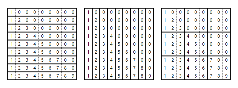
9 X 9 격자를 다루는 상황에서 위의 각 묶여진 셀들에 대해 연산을 하고싶다고 하자, 각 묶여진 공간끼리는 독립적이므로 vmap을 사용하는 것이 유리할 것이다.
여기서는 연산을 jnp.sum이라고 하자. (물론 jnp.sum은 axis를 통해 행, 열 방향으로 sum을 할 수 있지만 여기서는 그런 함수가 아니라 가정하자, 물론 jnp.sum으로도 3번째 예시를 한번에 구하는 방법은 없다.)
일단 첫번째 예시는 쉽게 구할 수 있을 것이다.
1
2
3
4
5
6
7
8
9
10
11
array = jnp.array([
    [1, 0, 0, 0, 0, 0, 0, 0, 0],
    [1, 2, 0, 0, 0, 0, 0, 0, 0],
    [1, 2, 3, 0, 0, 0, 0, 0, 0],
    [1, 2, 3, 4, 0, 0, 0, 0, 0],
    [1, 2, 3, 4, 5, 0, 0, 0, 0],
    [1, 2, 3, 4, 5, 6, 0, 0, 0],
    [1, 2, 3, 4, 5, 6, 7, 0, 0],
    [1, 2, 3, 4, 5, 6, 7, 8, 0],
    [1, 2, 3, 4, 5, 6, 7, 8, 9]
])
1
2
jax.vmap(jnp.sum)(array)
# Array([ 1,  3,  6, 10, 15, 21, 28, 36, 45], dtype=int32)
그렇다면 두번째는 어떨까? 두번째는 행렬을 traspose하면 될 것이다. 혹은 in_axes=1로 하는 방법도 있다.
1
2
3
4
jax.vmap(jnp.sum)(array.T)
# Array([ 9, 16, 21, 24, 25, 24, 21, 16,  9], dtype=int32)
jax.vmap(jnp.sum, in_axes=1)(array)
# Array([ 9, 16, 21, 24, 25, 24, 21, 16,  9], dtype=int32)
세번째는 어떨까, 방법이 바로 떠오르지 않을 것이다. 방법을 찾아보면, 우리는 앞의 두 예시에서 우리가 연산하기를 원하는 범위를 vmap의 in_axes (보통 0) 에 해당하는 축의 각 요소로 넣어주었다. 즉 아래와 같다.
in_axes=0: 각 행(axis=0)이 내가 연산하기 원하는 요소가 된다.in_axes=1: 각 열(axis=1)이 내가 연산하기 원하는 요소가 된다.
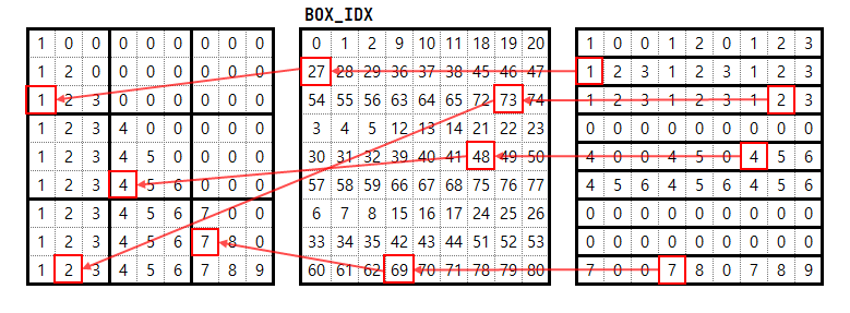
그렇다면 세번째는 어떻게 하면 될까? jnp.take를 활용하면 된다. jnp.take는 다음과 같다.
1
jax.numpy.take(a, indices, axis=None, ...)
Take elements from an array.
indices는 인덱스를 가지는 배열이고, 인덱스의 해당 위치에는 i라고 적혀있다고 하면 해당 위치의 값은 a[i] 이다.
그렇면 다음과 같은 하드코딩을 통해 vmap을 활용할 수 있다. jumanji의 코드를 참고하였다.
1
2
3
4
5
6
7
8
9
10
11
12
13
14
# jumanji/environments/logic/sudoku/constants.py
BOX_IDX = np.array(
    [
        [0, 1, 2, 9, 10, 11, 18, 19, 20],
        [27, 28, 29, 36, 37, 38, 45, 46, 47],
        [54, 55, 56, 63, 64, 65, 72, 73, 74],
        [3, 4, 5, 12, 13, 14, 21, 22, 23],
        [30, 31, 32, 39, 40, 41, 48, 49, 50],
        [57, 58, 59, 66, 67, 68, 75, 76, 77],
        [6, 7, 8, 15, 16, 17, 24, 25, 26],
        [33, 34, 35, 42, 43, 44, 51, 52, 53],
        [60, 61, 62, 69, 70, 71, 78, 79, 80],
    ]
)
그러면 다음과 같이 매핑된다.
1
2
3
4
5
6
7
8
9
10
jnp.take(array, jnp.asarray(BOX_IDX))
# Array([[1, 0, 0, 1, 2, 0, 1, 2, 3],
#        [1, 2, 3, 1, 2, 3, 1, 2, 3],
#        [1, 2, 3, 1, 2, 3, 1, 2, 3],
#        [0, 0, 0, 0, 0, 0, 0, 0, 0],
#        [4, 0, 0, 4, 5, 0, 4, 5, 6],
#        [4, 5, 6, 4, 5, 6, 4, 5, 6],
#        [0, 0, 0, 0, 0, 0, 0, 0, 0],
#        [0, 0, 0, 0, 0, 0, 0, 0, 0],
#        [7, 0, 0, 7, 8, 0, 7, 8, 9]], dtype=int32)
맨 오른쪽 격자의 맨 윗줄이 맨 왼쪽의 격자의 맨 왼쪽 위의 3 X 3 격자에 매핑되는 것을 쉽게 확인할 수 있을 것이다.
이러면 각 공간별로 vmap을 적용할 수 있다.
다시 원래대로 돌리는 index를 구하려면 jnp.argsort(BOX_IDX.flatten()).reshape(9, 9)를 사용하면 된다.
1
2
3
4
5
6
7
8
9
10
11
12
13
14
15
16
17
18
19
20
21
22
23
24
25
26
27
28
29
30
31
32
33
34
35
36
import numpy as np
import jax.numpy as jnp

array = jnp.array([
    [1, 0, 0, 0, 0, 0, 0, 0, 0],
    [1, 2, 0, 0, 0, 0, 0, 0, 0],
    [1, 2, 3, 0, 0, 0, 0, 0, 0],
    [1, 2, 3, 4, 0, 0, 0, 0, 0],
    [1, 2, 3, 4, 5, 0, 0, 0, 0],
    [1, 2, 3, 4, 5, 6, 0, 0, 0],
    [1, 2, 3, 4, 5, 6, 7, 0, 0],
    [1, 2, 3, 4, 5, 6, 7, 8, 0],
    [1, 2, 3, 4, 5, 6, 7, 8, 9]
])

BOX_IDX = jnp.array(
    [
        [0, 1, 2, 9, 10, 11, 18, 19, 20],
        [27, 28, 29, 36, 37, 38, 45, 46, 47],
        [54, 55, 56, 63, 64, 65, 72, 73, 74],
        [3, 4, 5, 12, 13, 14, 21, 22, 23],
        [30, 31, 32, 39, 40, 41, 48, 49, 50],
        [57, 58, 59, 66, 67, 68, 75, 76, 77],
        [6, 7, 8, 15, 16, 17, 24, 25, 26],
        [33, 34, 35, 42, 43, 44, 51, 52, 53],
        [60, 61, 62, 69, 70, 71, 78, 79, 80],
    ]
)

inverse_map = jnp.argsort(BOX_IDX.flatten()).reshape(9, 9)

array2 = jnp.take(array, BOX_IDX)
array3 = jnp.take(array2, inverse_map)

print(jnp.all(array == array3))
# True
참고로 아래 배열은 똑같이 3 X 3 공간에 대해 연산하는데도 불구하고, 변환 배열과 역변환 하는 배열이 같다. (위의 예시는 각 3 X 3 덩어리 9개라고 생각했을 때 (0, 0), (1, 0), (2, 0), (1, 0), …, (2, 2) 순서로 각 행에 배치되지만 아래는 (0, 0), (0, 1), (0, 2), (1, 0), …, (2, 2) 순서로 배치된다.)
1
2
3
4
5
6
7
8
9
10
11
12
13
14
15
16
17
BOX_IDX = jnp.array(
    [
        [0, 1, 2, 9, 10, 11, 18, 19, 20],
        [3, 4, 5, 12, 13, 14, 21, 22, 23],
        [6, 7, 8, 15, 16, 17, 24, 25, 26],
        [27, 28, 29, 36, 37, 38, 45, 46, 47],
        [30, 31, 32, 39, 40, 41, 48, 49, 50],
        [33, 34, 35, 42, 43, 44, 51, 52, 53],
        [54, 55, 56, 63, 64, 65, 72, 73, 74],
        [57, 58, 59, 66, 67, 68, 75, 76, 77],
        [60, 61, 62, 69, 70, 71, 78, 79, 80],
    ]
)

inverse_idx = jnp.argsort(BOX_IDX.flatten()).reshape(9, 9)
jnp.all(BOX_IDX == inverse_idx)
# Array(True, dtype=bool)
6. dynamic_slice, slice, indexing
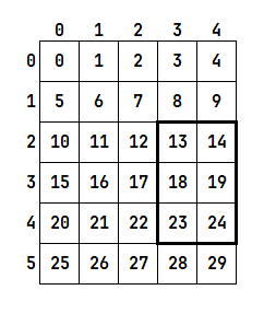
위와같이 (6, 5) shape를 가진 배열의 굵게 처리된 부분을 얻고 싶다고 한다면 세가지 방법이 있을 것이다.
jax.lax.dynamic_slicejax.lax.slice- indexing
1
2
3
4
5
6
7
8
9
10
def d_slice_3x2(arr, x, y):
    return jax.lax.dynamic_slice(arr, (x, y), (3, 2))

def slice_fn_3x2(arr, x, y):
    return jax.lax.slice(arr, (x, y), (x+3, y+2))

def slice_index_3x2(arr, x, y):
    return arr[x:x+3, y:y+2]

arr = jnp.arange(30).reshape(6, 5)
각 함수를 실행하면 결과는 다음과 같다.
1
2
3
4
5
6
7
8
print("d_slice")
print(d_slice_3x2(arr, 2, 3))

print("slice_fn")
print(slice_fn_3x2(arr, 2, 3))

print("slice_index")
print(slice_index_3x2(arr, 2, 3))
1
2
3
4
5
6
7
8
9
10
11
12
d_slice
[[13 14]
 [18 19]
 [23 24]]
slice_fn
[[13 14]
 [18 19]
 [23 24]]
slice_index
[[13 14]
 [18 19]
 [23 24]]
그렇다면 얻고자 하는 범위가 배열의 크기를 넘어가면 어떻게 될까? 예를 들어 다음과 같은 범위를 얻고 싶다고 가정하자.
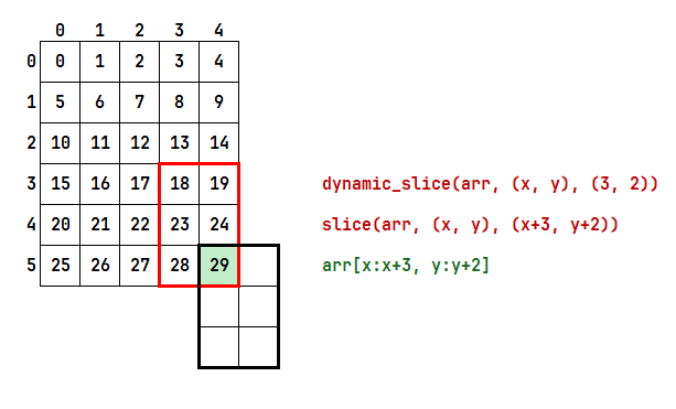
그럼 위 그림에도 나와있다시피 실행시 결과는 다음과 같이 나온다.
1
2
3
print(d_slice_3x2(arr, 5, 4))
print(slice_fn_3x2(arr, 5, 4))
print(slice_index_3x2(arr, 5, 4))
1
2
3
4
5
6
7
[[18 19]
 [23 24]
 [28 29]]
[[18 19]
 [23 24]
 [28 29]]
[[29]]
여기서 각 함수를 jitting 하면 결과가 다음과 같다.
1
jitted_d_slice_3x2(arr, 2, 3)
1
2
3
Array([[13, 14],
       [18, 19],
       [23, 24]], dtype=int32)
1
jitted_slice_fn_3x2(arr, 2, 3)
1
2
3
TracerArrayConversionError: The numpy.ndarray conversion method __array__() was called on traced array with shape int32[].
The error occurred while tracing the function slice_fn_3x2 at <ipython-input-4-6fbf264c417e>:4 for jit. This concrete value was not available in Python because it depends on the value of the argument x.
See https://jax.readthedocs.io/en/latest/errors.html#jax.errors.TracerArrayConversionError
1
jitted_slice_index_3x2(arr, 2, 3)
1
2
3
IndexError: Array slice indices must have static start/stop/step to be used with NumPy indexing syntax.
Found slice(Traced<ShapedArray(int32[], weak_type=True)>with<DynamicJaxprTrace(level=1/0)>, Traced<ShapedArray(int32[], weak_type=True)>with<DynamicJaxprTrace(level=1/0)>, None).
To index a statically sized array at a dynamic position, try lax.dynamic_slice/dynamic_update_slice (JAX does not support dynamically sized arrays within JIT compiled functions).
dynamic_slice 만 가능하다. 아직 정확한 이유는 파악하기 어렵지만 dynamic_slice는 함수 호출시에 반환되는 배열의 크기를 확정할 수 있기 때문인 것으로 보인다.
DynamicSlice에 대한 XLA 공식 문서에는 다음과 같이 적혀있다. (사실상 JAX와 같다)
DynamicSlice(operand, start_indices, size_indices)
The effective slice indices are computed by applying the following transformation for each index i in [1, N) before performing the slice:
1
start_indices[i] = clamp(start_indices[i], 0, operand.dimension_size[i] - size_indices[i])
This ensures that the extracted slice is always in-bounds with respect to the operand array. If the slice is in-bounds before the transformation is applied, the transformation has no effect.
start_indices가 clamp 연산된다는 것을 이해하면 방금 (5, 4)에서 인덱싱한 결과가 왜 저렇게 나왔는지 이해가 될 것이다.
7. functools.partial 활용하기
직접올린 JAX의 Discussion Q&A를 재구성하였다.
일단 functools.partial에 대해 이해해보자
functools.partial 공식문서에서는 다음과 같이 설명하고 있다.
Return a new partial object which when called will behave like func called with the positional arguments args and keyword arguments keywords. If more arguments are supplied to the call, they are appended to args. If additional keyword arguments are supplied, they extend and override keywords. Roughly equivalent to:
새로운 partial 객체를 반환하며, 호출 시에 args라는 위치 인자와 keywords라는 키워드 인자를 사용하여 func가 호출된 것처럼 동작합니다. 호출 시에 더 많은 인자가 제공되면 그것들은 args에 추가됩니다. 추가적인 키워드 인자가 제공되면, 그것들은 keywords를 확장하거나 덮어씁니다. 이는 대략적으로 다음과 동등합니다:
1
2
3
4
5
6
7
8
def partial(func, /, *args, **keywords):
    def newfunc(*fargs, **fkeywords):
        newkeywords = {**keywords, **fkeywords}
        return func(*args, *fargs, **newkeywords)
    newfunc.func = func
    newfunc.args = args
    newfunc.keywords = keywords
    return newfunc
The partial() is used for partial function application which “freezes” some portion of a function’s arguments and/or keywords resulting in a new object with a simplified signature. For example, partial() can be used to create a callable that behaves like the int() function where the base argument defaults to two:
partial() 함수는 함수의 인자나 키워드 중 일부를 “고정”하여 간소화된 서명(signature)을 가진 새로운 객체(object)를 생성하는 데 사용됩니다. 예를 들어, partial()을 사용하면 int() 함수처럼 동작하되, base 인자를 기본값으로 2로 설정한 호출 가능한 객체를 만들 수 있습니다.
1
2
3
4
5
>>> from functools import partial
>>> basetwo = partial(int, base=2)
>>> basetwo.__doc__ = 'Convert base 2 string to an int.'
>>> basetwo('10010')
18
예시를 하나만 더 들면 다음과 같다.
1
2
3
4
5
6
7
8
9
10
11
12
13
14
import functools


def cal(x, y, z):
    return x * y + z


cal_ver1 = functools.partial(cal, x=3, z=2)
cal_ver2 = functools.partial(cal, 3, 2)

print(cal_ver1(y=5))
# print(cal_ver1(3)) # 오류 : 3은 왼쪽부터 채워져 x=3으로 취급됨, 중복인자
print(cal_ver2(5))  # 3, 2가 왼쪽부터 채워져 x=3, y=2, z=5 로 취급됨.
functools.partial에 func를 제외하고 positional arguments를 입력할지 keyword arguments로 입력할지 잘 선택해야 한다. positional arguemnts로 입력시 왼쪽부터 채워지며 keyword arguments로 입력시 해당 키워드에 맞게 채워진다.
functools.partial에 대해 설명하였다. 나는 이것을 다음과 같이 활용하였다. 아래 내용은 실제 문제를 상당히 간소화한 버전이다.
1
2
3
4
5
6
7
8
9
10
11
12
13
14
15
16
@jax.jit
def get_result(x):
    fn_list = (
        lambda x: x + 1,
        lambda x: x + 2,
        lambda x: x + 3,
    )

    def add_number(fn_index, x):
        return jax.lax.switch(fn_index, fn_list, x)

    result = jax.lax.fori_loop(0, len(fn_list), add_number, x)
    return result

get_result(4)
# Array(10, dtype=int32, weak_type=True)
fn_list가 있고 각 iteration 마다 적용하기 위한 함수가 저장되어 있었고 각 iteration마다 해당 fn을 실행해야 했다. 하지만 해당 fn 연산은 add_number에서 상당히 많이 이루어지고 그리고 x에만 적용하는 것이 아니고 다른 변수에도 적용할 수 있기 때문에 계속해서 적용할 방법이 필요했다.
그렇다고 매번 jax.lax.switch를 쓰자니 코드가 너무 지저분했다.
이럴 경우 functools.partial을 활용할 수 있다.
1
2
3
4
5
6
7
8
9
10
11
12
13
14
15
16
17
@jax.jit
def get_result_partial(x):
    fn_list = (
        lambda x: x + 1,
        lambda x: x + 2,
        lambda x: x + 3,
    )

    def add_number(fn_index, x):
        fn = functools.partial(jax.lax.switch, fn_index, fn_list)
        return fn(x)

    result = jax.lax.fori_loop(0, len(fn_list), add_number, x)
    return result

get_result_partial(4)
# Array(10, dtype=int32, weak_type=True)
위와같이 jax.lax.switch 활용시 fn_index, fn_list는 계속 고정되니 해당 연산을 functools.partial를 이용하여 변수에 따로 저장할 수 있다.
8. lax.select, lax.cond
lax.cond의 문서를 살펴보면 다음과 같은 내용이 있다.
In contrast with jax.lax.select(), using cond indicates that only one of the two branches is executed (up to compiler rewrites and optimizations). However, when transformed with vmap() to operate over a batch of predicates, cond is converted to select().
위 내용 중 only one of the two branches is excuted 부분을 실험해 보려고 한다.
실험 방법은 다음과 같다.
- 연산 대상 배열의 크기가 큰 것과 작은 것
- 연산량이 큰 연산과 작은 연산
- True/False
각각 조합하면 8개가 나온다. 다음과 같은 코드로 연산한다.
코드에 나와있다시피 True일 경우 x와 x의 내적을 구하고, False일 경우 x에 1을 더한다. 즉 True일 경우 연산량이 크고, False일 경우 연산량이 작다.
1
2
3
4
5
6
7
8
9
10
11
12
13
14
15
16
17
18
19
20
21
22
@jax.jit
def cond_fn(c, x):
    return jax.lax.cond(c, lambda x: jnp.dot(x, x), lambda x: x+1, x)

@jax.jit
def select_fn(c, x):
    return jax.lax.select(c, jnp.dot(x, x), x+1)


arr_small = jnp.ones((10, 10))
arr_large = jnp.ones((10000, 10000))

# warming up
cond_fn(True, arr_small)
cond_fn(False, arr_small)
select_fn(True, arr_small)
select_fn(False, arr_small)

cond_fn(True, arr_large)
cond_fn(False, arr_large)
select_fn(True, arr_large)
select_fn(False, arr_large)
cond_fn과 select_fn의 결과는 같다.
시간 측정은 다음과 같이 하였다.
1
2
3
%%timeit

<cond/select>_fn(<True/False>, arr_<small/large>).block_until_ready()
각 연산 결과는 다음과 같다. 절대적 수치보다는 상대적 수치에 주목하자
| arr_small | arr_small | arr_large | arr_large | |
|---|---|---|---|---|
| TRUE | FALSE | TRUE | FALSE | |
| cond_fn | 38 | 34.6 | 26100 | 1100 |
| select_fn | 33.7 | 32.5 | 27200 | 27300 |
결과는 다음과 같다.
- 연산량이 적을 경우
lax.select가 더 빠르다. lax.cond는 확실히 한 분기만 실행하는 것처럼 보인다.lax.select의 경우 모든 경우에서 연산량이 거의 차이가 없다. 하지만lax.cond의 경우True일 경우 연산량이 크고,False일 경우 연산량이 작다. 이는lax.cond가 한 분기만 실행하는 것을 보여준다.
연산량이 적을 경우 lax.select가 더 빠른 것에 대하여 make_jaxpr을 살펴보았다.
1
make_jaxpr(cond_fn)(True, arr_small)  # True/False 가 결과가 같다.
1
2
3
4
5
6
7
8
9
10
11
12
13
14
15
16
17
18
19
20
{ lambda ; a:bool[] b:f32[10,10]. let
    c:f32[10,10] = pjit[
      name=cond_fn
      jaxpr={ lambda ; d:bool[] e:f32[10,10]. let
          f:i32[] = convert_element_type[new_dtype=int32 weak_type=False] d
          g:f32[10,10] = cond[
            branches=(
              { lambda ; h:f32[10,10]. let i:f32[10,10] = add h 1.0 in (i,) }
              { lambda ; j:f32[10,10]. let
                  k:f32[10,10] = dot_general[
                    dimension_numbers=(([1], [0]), ([], []))
                    preferred_element_type=float32
                  ] j j
                in (k,) }
            )
            linear=(False,)
          ] f e
        in (g,) }
    ] a b
  in (c,) }
1
make_jaxpr(select_fn)(True, arr_small)
1
2
3
4
5
6
7
8
9
10
11
12
13
{ lambda ; a:bool[] b:f32[10,10]. let
    c:f32[10,10] = pjit[
      name=select_fn
      jaxpr={ lambda ; d:bool[] e:f32[10,10]. let
          f:f32[10,10] = dot_general[
            dimension_numbers=(([1], [0]), ([], []))
            preferred_element_type=float32
          ] e e
          g:f32[10,10] = add e 1.0
          h:f32[10,10] = select_n d g f
        in (h,) }
    ] a b
  in (c,) }
lax.cond의 경우 jaxpr에 branches가 나타나있다. 이 부분에서 연산이 생기기 때문에 이 연산보다 다른 분기 연산이 더 작을 경우 lax.select가 더 빠른 것으로 보인다.
하지만 lax.cond의 경우 vmap을 사용할 경우 lax.select로 변환된다. 이 부분도 구현시 고려해야 할 것이다.